library(sf)         # for spatial data handling
library(forcats)    # for factor handling
library(dplyr)      # for data manipulation
library(ggplot2)    # for generic plotting
library(rpart)      # for building the model
library(rpart.plot) # for plotting the model
library(tmap) # for spatial maps2 Data Description
2.1 Original Dataset
The original dataset provided by Zheng et al. (2011) was collected in the GeoLife project (Microsoft Research Asia) by 182 users in a period of over three years (from April 2007 to August 2012). A GPS trajectory of this dataset is represented by a sequence of time-stamped points, each of which contains the information of latitude, longitude and altitude. This dataset contains 17’621 trajectories with a total distance of about 1.2 million kilometers and a total duration of 48,000+ hours. These trajectories were recorded by different GPS loggers and GPS-phones, and have a variety of sampling rates. 91 percent of the trajectories are logged in a dense representation, e.g. every 1~5 seconds or every 5~10 meters per point.
This dataset consists of a broad range of users’ outdoor movements, including not only life routines like go home and go to work but also some entertainments and sports activities, such as shopping, sightseeing, dining, hiking, and cycling. 73 users have labeled their trajectories with transportation mode, such as driving, taking a bus, riding a bike and walking.
2.2 Processed dataset
We downloaded Version 1.2.2 of the original dataset (on the 19.11.2024) and processed it in the following manner:
- Merged the data of all users into a single dataset
- Added transport mode labels and removed all trajectories without a transport mode label.
- Split the trajectories into segments based on the user id, transportation mode and time difference between consecutive points. A new segment is created if the time difference is larger than 10 minutes.
- Split the segments (from the previous step) further based on the distance between consecutive points. A new segment is created if the distance is larger than 100 meters. The created segment ids are unique across all users.
- Removed all segments with less than 100 points.
- Projected the data into UTM zone 50N (EPSG: 32650)
- Removed all segments that move outside of the bounding box of Beijing (406993 , 487551 , 4387642, 4463488 in EPSG 32650)
- Split the data into 4 sets of training, testing and validation data.
The full process is documented in this GitHub Repository.
2.3 Feature-enriched dataset
For this exercise, we provide preprocessed data files (tracks_*_processed.gpkg) with pre-calculated movement features. These features were computed at the point level from the raw GPS trajectories:
2.3.1 Available features
steplength (numeric): Distance between consecutive GPS points in meters. Calculated as the Euclidean distance between point \(i\) and point \(i+1\).
timelag (numeric): Time difference between consecutive points in seconds. Calculated as the temporal difference between point \(i\) and point \(i+1\).
speed (numeric): Instantaneous movement speed in meters per second (m/s). Calculated as: \[\text{speed} = \frac{\text{steplength}}{\text{timelag}}\]
acceleration (numeric): Rate of change in speed in meters per second squared (m/s²). Calculated as: \[\text{acceleration} = \frac{\text{speed}_{i+1} - \text{speed}_i}{\text{timelag}_i}\]
sinuosity (numeric): Path curvature measured over a 5-point observation window. Calculated as the ratio of actual distance traveled to straight-line distance: \[\text{sinuosity} = \frac{\sum_{j=0}^{4} \text{steplength}_{i+j}}{\text{straight\_distance}(point_i, point_{i+5})}\] where a value of 1 indicates a perfectly straight path and higher values indicate more winding paths.
2.3.2 Data import and visualisation
Download the dataset tracks_1_processed.gpkg from moodle.
To import and visualize the data we suggest the following libraries in R. Feel free to use different programming languages / libraries. If you want to follow along with our code, install the libraries below using install.packages().
The dataset tracks_1_processed.gpkg contains the training and testing data as separate layers.
# List layers in the geopackage
st_layers("data/tracks_1_processed.gpkg")
Driver: GPKG
Available layers:
layer_name geometry_type features fields crs_name
1 training Point 501432 11 WGS 84 / UTM zone 50N
2 testing Point 262851 11 WGS 84 / UTM zone 50N
3 validation Point 240449 10 WGS 84 / UTM zone 50Ntraining_dataset <- read_sf("data/tracks_1_processed.gpkg", layer = "training") |>
mutate(data = "training")
testing_dataset <- read_sf("data/tracks_1_processed.gpkg", layer = "testing") |>
mutate(data = "testing")
full_dataset <- bind_rows(training_dataset, testing_dataset)
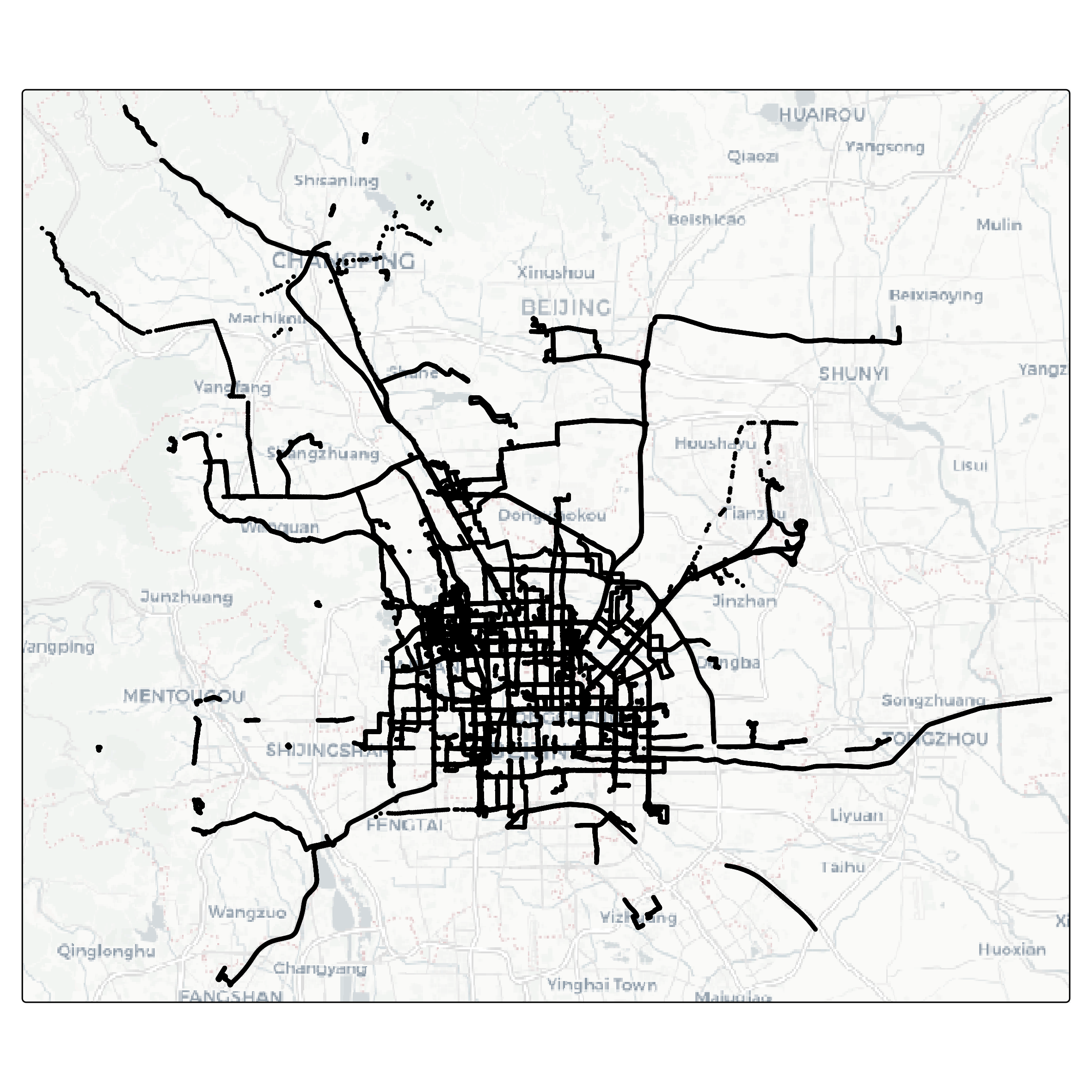
full_dataset$mode <- as.factor(full_dataset$mode)Let’s visualize the data as a map. The package tmap is very handy for this task.
overview <- full_dataset |>
  tm_shape() +
  tm_dots(fill = "mode") +
  tm_facets("mode", ncol = 3, free.coords = FALSE) +
  tm_basemap("CartoDB.Positron") +
  tm_layout(legend.show = FALSE)

tmap_save(overview, "overview.png", width = 30, height = 20, units = "cm")